
 RSS Feed
Blog > Post
Cloud-Based Analytics With SingleStoreDB
von Akmal Chaudhri, SingleStore (sponsor) , 9. Juni 2022
Tags:
Create Cloud Accounts
Create a SingleStore Cloud Account
First, we’ll create a free Cloud account on the SingleStore website. At the time of writing, the Cloud account from SingleStore comes with a $500 credit. We’ll create our cluster and note the host address and password as we’ll need this information later.
We’ll use the SQL Editor to create two new databases, as follows:
CREATE DATABASE IF NOT EXISTS btc_db;
Create a MindsDB Cloud Account
Next, we’ll create a free Cloud account on the MindsDB website. We’ll note our login email address and password as we’ll need this information later.
Create a Deepnote Account
Finally, we’ll create a free account on the Deepnote website. Once logged in, we’ll create a Deepnote MindsDB integration, as shown below:
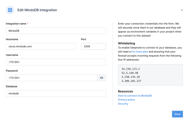
- Integration name: MindsDB
- Hostname: cloud.mindsdb.com
- Port: 3306
- Username: TO DO
- Password: TO DO
- Database: mindsdb
The TO DO for Username and Password should be replaced with the login values for MindsDB Cloud. We’ll use mindsdb for the Database name.
We’ll now create a new Deepnote project which will give us a new notebook. We’ll add the MindsDB integration to the notebook.
In our Deepnote project, we’ll create two sub-directories, /csv and /jar, to store CSV data files and JAR files, respectively.
1. Apache Spark
Apache Spark is an open-source engine for analytics and data processing. Spark can utilise the resources of a cluster of machines to execute operations in parallel with fault tolerance. A great way to test Spark without installing it locally is by using Deepnote. Deepnote provides instructions for installing Spark and offers a notebook environment that allows Exploratory Data Analysis (EDA), all entirely cloud-based. This would be perfect for many use-cases.
Let’s look at how we could load some data into Deepnote, perform some data analysis and then write the data into SingleStoreDB.
After creating a project in Deepnote, we can use the SingleStoreDB Spark Connector — rather than using SQLAlchemy or JDBC directly.The SingleStoreDB Spark Connector provides many benefits, including:
- Implements as a native Spark SQL plugin
- Accelerates ingest from Spark via compression
- Supports data loading and extraction from database tables and Spark Dataframes
- Integrates with the Catalyst query optimiser and supports robust SQL Pushdown
- Accelerates machine-learning (ML) workloads
We need three jar files uploaded into our project directory in Deepnote:
- singlestore-jdbc-client-1.0.1.jar
- singlestore-spark-connector_2.12–4.0.0-spark-3.2.0.jar
- spray-json_3–1.3.6.jar
We'll use the Iris flower data set for a quick and simple example of data that we could load into SingleStoreDB. We can obtain the CSV file data and upload it into our project directory in Deepnote.
Next, we’ll need to install PySpark from our notebook:
! sudo mkdir -p /usr/share/man/man1
! sudo apt-get install -y openjdk-11-jdk
! pip install pyspark==3.2.1
and then we can prepare our SparkSession:
spark = (SparkSession
.builder
"spark.jars",
"jars/singlestore-jdbc-client-1.0.1.jar, \
jars/spray-json_3-1.3.6.jar"
)
.getOrCreate() )
We can check the version of Spark as follows:
The output should be:
Next, let’s provide connection details for SingleStore DB:
password = "TO DO"
port = "3306"
cluster = server + ":" + port
The TO DO for server and password should be replaced with the values obtained from SingleStoreDB Cloud when creating a cluster. We’ll now set some parameters for the Spark Connector:
We can now create a new Spark Dataframe from our Iris CSV data file:
and we can view the data:
The output should be similar to the following:
|sepal_length|sepal_width|petal_length|petal_width| species|
+------------+-----------+------------+-----------+-----------+
| 5.1| 3.5| 1.4| 0.2|Iris-setosa|
| 4.9| 3.0| 1.4| 0.2|Iris-setosa|
| 4.7| 3.2| 1.3| 0.2|Iris-setosa|
| 4.6| 3.1| 1.5| 0.2|Iris-setosa|
| 5.0| 3.6| 1.4| 0.2|Iris-setosa|
+------------+-----------+------------+-----------+-----------+
only showing top 5 rows
.groupBy("species")
.count()
.show()
)
The output should be similar to the following:
+---------------+-----+
| species|count|
+---------------+-----+
| Iris-virginica| 50|
| Iris-setosa| 50|
|Iris-versicolor| 50|
+---------------+-----+
We have three different species of flowers with 50 records each.
We can also find additional information as follows:
.describe(
"sepal_length",
"sepal_width",
"petal_length",
"petal_width"
)
.show()
)
The output should be similar to the following:
+-------+-------------+------------+-------------+------------+
|summary| sepal_length| sepal_width| petal_length| petal_width|
+-------+-------------+------------+-------------+------------+
| count| 150| 150| 150| 150|
| mean| 5.8433333333| 3.054000000|3.75866666666|1.1986666666|
| stddev|0.82806612797|0.4335943113|1.76442041995|0.7631607417|
| min| 4.3| 2.0| 1.0| 0.1|
| max| 7.9| 4.4| 6.9| 2.5|
+-------+-------------+------------+-------------+------------+
We can also create a PCA visualization using an example from Plotly:
import plotly.express as px
from sklearn.decomposition import PCA
import pandas as pd
pandas_iris_df = iris_df.toPandas()
X = pandas_iris_df"sepal_length", "sepal_width", "petal_length", "petal_width"
pca = PCA(n_components = 2)
components = pca.fit_transform(X)
pca_fig = px.scatter(
components,
x = 0,
y = 1,
color = pandas_iris_df["species"]
)
pca_fig.show()
The output should be similar to the following: 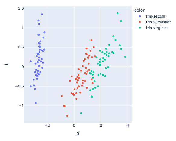
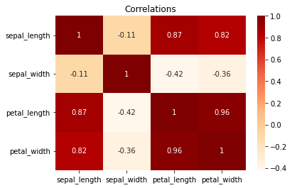
Further analysis could include finding correlations, for example:
import matplotlib.pyplot as plt
sns.heatmap(
pandas_iris_df.corr(),
cmap = "OrRd",
annot = True
)
plt.plot()
The output should be similar to to the following figure.
And even further research is possible. There are numerous possibilities.
We can slice and dice the data in this interactive cloud-based environment, perform various analyses, build charts, graphs and more. When we are ready, we can save our data into SingleStoreDB:
.format("singlestore")
.option("loadDataCompression", "LZ4")
.mode("overwrite")
.save("iris_db.iris")
)
Next, let’s look at how we could use Machine Learning (ML) in the cloud with SingleStoreDB.
2. MindsDB
MindsDB is an example of an AutoML tool with support for in-SQL machine learning . It can seamlessly integrate with SingleStoreDB. Let’s explore how.
We’ll adapt a Time-series forecasting example for Bitcoin. We can obtain the CSV file data and upload it into our project directory in Deepnote.
First, we’ll define our Spark Dataframe schema:
btc_schema = StructType([
StructField("ds", DateType(), True),
StructField("y", FloatType(), True)
])
Next, we’ll read the CSV file data into a Spark Dataframe using the schema we just defined:
"data/btc_data.csv",
header = True,
dateFormat = "YYYY-MM-DD",
schema = btc_schema
)
and we can view the data:
The output should be similar to the following:
+----------+---------+| ds| y|
+----------+---------+
|2011-12-31| 4.471603|
|2012-01-01| 4.71|
|2012-01-02| 5.0|
|2012-01-03| 5.2525|
|2012-01-04|5.2081594|
+----------+---------+
only showing top 5 rows
Our time-series data consists of the Bitcoin price (y) on a particular date (ds).
We’ll now save our data into SingleStoreDB:
.format("singlestore")
.option("loadDataCompression", "LZ4")
.mode("overwrite")
.save("btc_db.btc")
)
The following cell should be run if this particular Minds DBDATASOURCE was previously created:
and then we’ll create the DATASOURCE:
WITH ENGINE = "singlestore",
PARAMETERS = {
"user" : "admin",
"password" : "TO DO",
"host" : "TO DO",
"port" : 3306,
"database" : "btc_db"
}
The TO DO for password and host should be replaced with the values obtained from SingleStoreDB Cloud when creating a cluster.
We can now view the table contents:
FROM btc_data.btc
ORDER BY ds
LIMIT 5;
The output should be similar to the following:
+------------+---------+
| ds | y |
+------------+---------+
| 2011-12-31 | 4.4716 |
| 2012-01-01 | 4.71 |
| 2012-01-02 | 5.0 |
| 2012-01-03 | 5.2525 |
| 2012-01-04 | 5.20816 |
+------------+---------+
5 rows in set
We want to build a model that predicts the price (y). Let’s create our predictor.
The following cell should be run if the PREDICTOR was previously created:
and we’ll create a new PREDICTOR:
FROM btc_data
(SELECT * FROM btc)
PREDICT y
ORDER BY ds
WINDOW 1;
In this first model-building iteration, we’ll use the WINDOW value set to 1. This will use the last row for every prediction. We can see the status by running and re-running the following command:
The status field will change from generating ➔ training ➔ complete. Once complete, we can get the actual and predicted Bitcoin prices as follows:
orig_table.y AS actual_y
FROM btc_data.btc AS orig_table
JOIN mindsdb.btc_pred AS pred_table
WHERE orig_table.ds > '2011-12-30'
LIMIT 10;
The output should be similar to the following:
+------------+--------------------+----------+
| date | predicted_y | actual_y |
+------------+--------------------+----------+
| 2020-09-14 | 10388.046619416727 | 10314.3 |
| 2020-09-13 | 10337.436201070366 | 10409.8 |
| 2020-09-12 | 10298.611981465672 | 10363.9 |
| 2020-09-11 | 10275.237535814897 | 10299.2 |
| 2020-09-10 | 10157.706201274084 | 10329.1 |
| 2020-09-09 | 10163.48052954538 | 10161.5 |
| 2020-09-08 | 10156.737703604405 | 10175.6 |
| 2020-09-07 | 10209.844514505841 | 10159.2 |
| 2020-09-06 | 10335.93543291758 | 10178.4 |
| 2020-09-05 | 10588.904678141687 | 10324.6 |
+------------+--------------------+----------+
10 rows in set
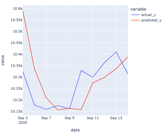
and a quick way to view this tabular result would be to create a plot:
pred_10_df,
x = "date",
y = ["actual_y", "predicted_y"]
)
line_fig.show()
An example of the output this may produce is shown below.
To make a new prediction, we can use the following:
orig_table.y AS actual_y
FROM btc_data.btc AS orig_table
JOIN mindsdb.btc_pred AS pred_table
WHERE orig_table.ds > LATEST;
The output should be similar to the following:
| date | predicted_y | actual_y |
+------------+-------------------+----------+
| 2020-09-14 | NULL | 10314.3 |
| NULL | 7537.247701719254 | NULL |
+------------+-------------------+----------+
2 rows in set
We could also now save all the predictions into SingleStoreDB for future use. First, we’ll need to get all the predictions, rather than just 10:
orig_table.y AS actual_y
FROM btc_data.btc AS orig_table
JOIN mindsdb.btc_pred AS pred_table
WHERE orig_table.ds > '2011-12-30';
Then, we’ll create a new Spark Dataframe:
and write the Dataframe to SingleStoreDB:
.format("singlestore")
.option("loadDataCompression", "LZ4")
.mode("overwrite")
.save("btc_db.pred")
)
Summary
This article has shown two quick examples of how easily SingleStoreDB can integrate with other modern technologies to provide a smooth development workflow. In both cases, we developed our solutions entirely in the cloud.
The SingleStoreDB Spark Connector provides a seamless experience when working with Spark Dataframes. We can read and write Spark Dataframes directly without converting them to other data representations, and do not need to use cursors or loops.
The MindsDB integration provides developers with the ability to build ML models quickly using the familiar SQL language syntax.
About the Author: |
Akmal Chaudhri is a Senior Technical Evangelist at SingleStore. Based in London, Akmal’s career spans work with database technology, consultancy, product strategy, technical writing, technical training and more. Through his work, Akmal helps build global developer communities and raise awareness of technology. |
Teilen sie diese Seite mit ihrem Netzwerk


